Mitch Richling: Growing 3D Trees

Many living things in nature, and a few non-living ones, grow by slowly aggregating material in a controlled way onto existing structures. In addition, a great many more natural structures that do not physically grow in this manner do have a have a final geometric form that may be approximated by a growth mechanism utilizing only controlled aggregation.

For example, consider the way a stalagmite grows on a cave floor. Over time, slightly acidic water drips down from the ceiling above carrying tiny amounts of dissolved rock - normally limestone. Some of this dissolved mineral drops from solution, and adheres to the face of the stalagmite. In this way, the stalagmite grows in layers by slowly aggregating material on top of material previously deposited in the same manner. Over time the mineral content of the water will have different compositions leading to the colorful, tree-like growth rings visible when lapidaries cut stalagmites into thin sections.

An excellent example of a living process growing through aggregation are several species of ocean coral. In the case of many corals, millions of individuals living in the community aggregate calcium deposits on top of the deposits already put down by the previous generation. Frequently this aggregation is quite patterned in that new material is only deposited on top of recently produced material leading to the tree like structure in many corals.

As another example, we may consider fungi. A large class of fungi, if you look closely enough, are made up of a branched mass of hyphae. Each hypha is shaped like a long, thin tube and contains many of the structures one would expect to find in a cell. All growth in these fungi occurs when a hyphal strand is extended at the tip or branches a small distance back from the growth tip. In this way a fungus can grow into a globular mass of small, branching fibers. Note that this is not purely aggregation onto a previous surface, but the final structure may be successfully modeled in this way.

As a final example, we consider a system with a more complex pattern of aggregation – an oak tree. One might think of tree trunks and limbs as growing by adding layers of new material on top of the of the old core material - and thus forming the familiar growth rings found inside tree trunks. But trees do more than just get thicker, they get longer – and they get longer FASTER than they get thicker. This means that any aggregation pattern must be non-uniform based upon where it occurs on the tree limb. To complicate matters even more, some limbs grow faster than others while some limbs just stop growing all together. All of this complexity, and we haven't even touched upon the most complex aspect of tree growth. Branching! In summary, the geometric pattern of aggregation in tree growth is quite complex, and exceptionally difficult to realistically model with a computer program.

A great simplifying assumption to this potentially horrifyingly complex geometric problem is to assume that everything is a sphere. We start with a sphere, and assume that the final result of an aggregation operation on that sphere is the union of the original sphere and a new sphere with a slightly different center. Thus the final product would be a union of spheres. Sounds too simple to model complex objects? Too simple to model the complex shape of a tree? Well, this page is devoted to demonstrating some of the complexity that can result from this simplification. Here is an example of what may be achieved:

First Example

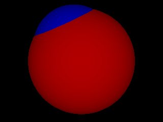
Let's dig into the concept introduced in the previous section. Consider for a moment if one had a spherical mass of biological material with the ability to produce new growth on it's surface. A good example might be a flower bulb. Further consider that this mass of biological material doesn't simply grow uniformly across the surface of the sphere. This could be because the life form in question only "wants" to grow a particular way, or because of some environmental condition. Next suppose this growth after a small time produces a "bump" of new material that looks like a circular patch that is thickest in the center. The picture below illustrates the initial sphere in red and the new growth, after some small time interval, in blue. Now imagine that this blue bump is really just the visible portion of a smaller blue sphere with a slightly different center than the original red sphere - so growth is simply the process of adding a new sphere to the system!

If we continue to add spheres of the same radius as the original blue one and offset in the same direction, then the result would be a cylinder protruding from the red sphere with a rounded off top. On the other hand, if the diameters of the new spheres linearly decreased as the offset grew, then the blue growth would end up looking like a cone. So we have two variables to control:

• The path along which growth occurs. Practically speaking, this amounts to computing the offset from the sphere added at the previous growth step.
• The radius of each new sphere. This controls the shape profile of the growing limb. Practically this amounts to computing the delta in size from the previous growth step.

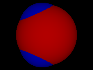
Simple! Now that we can grow a single limb, the next step is to consider what happens if growth appears in two different directions at the same time as illustrated in the image below.

If such growth were to continue we would get a pair of cylinders joined at the initial, red sphere. If the growth regions shrank as it grew, we would get two cone-like limbs attached to the initial sphere. This is very much like the fork found in a tree branch or in a fungal hypha. To grow trees, we need to algorithmically define how branching occurs, and thus we have added a new aspect to the model:

• Pragmatically determine when to add new limbs to the system.

All we need to do now is take the previous observations and develop a concrete algorithm from them. The core idea for a single limb, iterative algorithm should be immediate:

1. We begin with a single growth sphere.
2. We create a new growth sphere with a new radius and center both only slightly different from the current sphere, and mark the current sphere as dead.
3. Go back to step 2 (using the last added growth sphere).

Growing a single limb is simple, but we want a tree with branches. Branching translates into having TWO spheres from which we grow in step 2 of our algorithm above. So, all we must do is add to the algorithm the ability to occasionally generate two new spheres instead of one. Our new algorithm looks like this:

1. We begin with a collection of "growth spheres" – the spheres from which new growth springs.
2. For each growth sphere, we create a new growth sphere with a new radius and center both only slightly different from the current sphere; and mark the old sphere as dead.
3. We select from the set of dead spheres some that we will bring back to life and make growth spheres again – they will form the branch points for new limbs.
4. Go back to step 2.

The shape of the final result will be completely determined by the rules we use for the three decision points in the code: how we decide when to branch, the path new branches take, and the radius of new growth spheres along new branches. Now we just need rules for these three decision points!

For inspiration, consider real trees. Real tree branches generally don't grow toward each other, and they tend to grow toward the sun (or away from the earth). We can place energy functions in the space with our growing tree and pick new center points to minimize total energy to simulate this kind of behavior. For example, we can think of each growth sphere as a positively charged sphere and place a large positive "earth" in the direction we want the tree to grow away from. I implemented the idea above in a simple C program, and the image below is first result:

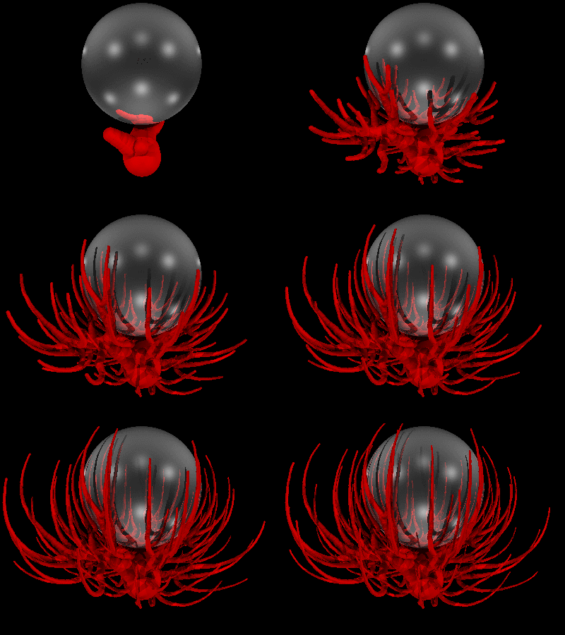
The effects possible by using different methods to pick direction and sphere size can be interesting. Consider the image below. Do you see the tree here? It's the base of the crystal ball!

The previous image was actually generated with a dramatically more sophisticated program. I have a long standing interest in autonomous systems, artificial life and artificial Intelligence. As it turns out the algorithm above can be completely, and naturally, described as the action of a swarm of autonomous, artificial life forms. For example, growth can be described as movement and branch points can be described as breeding. The coral reef analogy is actually very accurate in this formulation.

Any world simulator can be used for this kind of thing. I personally have been using several thousand lines of Java code implementing a custom world simulator for autonomous systems. It is quite a bit more general than most world simulators and has special support for several physical models. The physics that this world understands has been carefully implemented to be extended and overridden. The default, "Newtonian" type physics in this world, is not quite as simple as the real world. For example the universal gravitational force constant is modifiable for each object. This and many more rules of the universe are much more flexible in this program. In the world that generated the image below, the potential fields in the world were 3D, while the movement strategies used by the autonomous life forms were coplanar. The "bubbles" were life forms that had freedom in all three dimensions.

The following 5 pictures were the first real "trees" generated by the Java world simulator. They were all generated from the SAME CODE with only different growth parameters given.

Check out the fractals & fungi sections of my reading list.