Mitch Richling: Hopalong Fractals
| Author: | Mitch Richling |
| Updated: | 2024-10-31 |
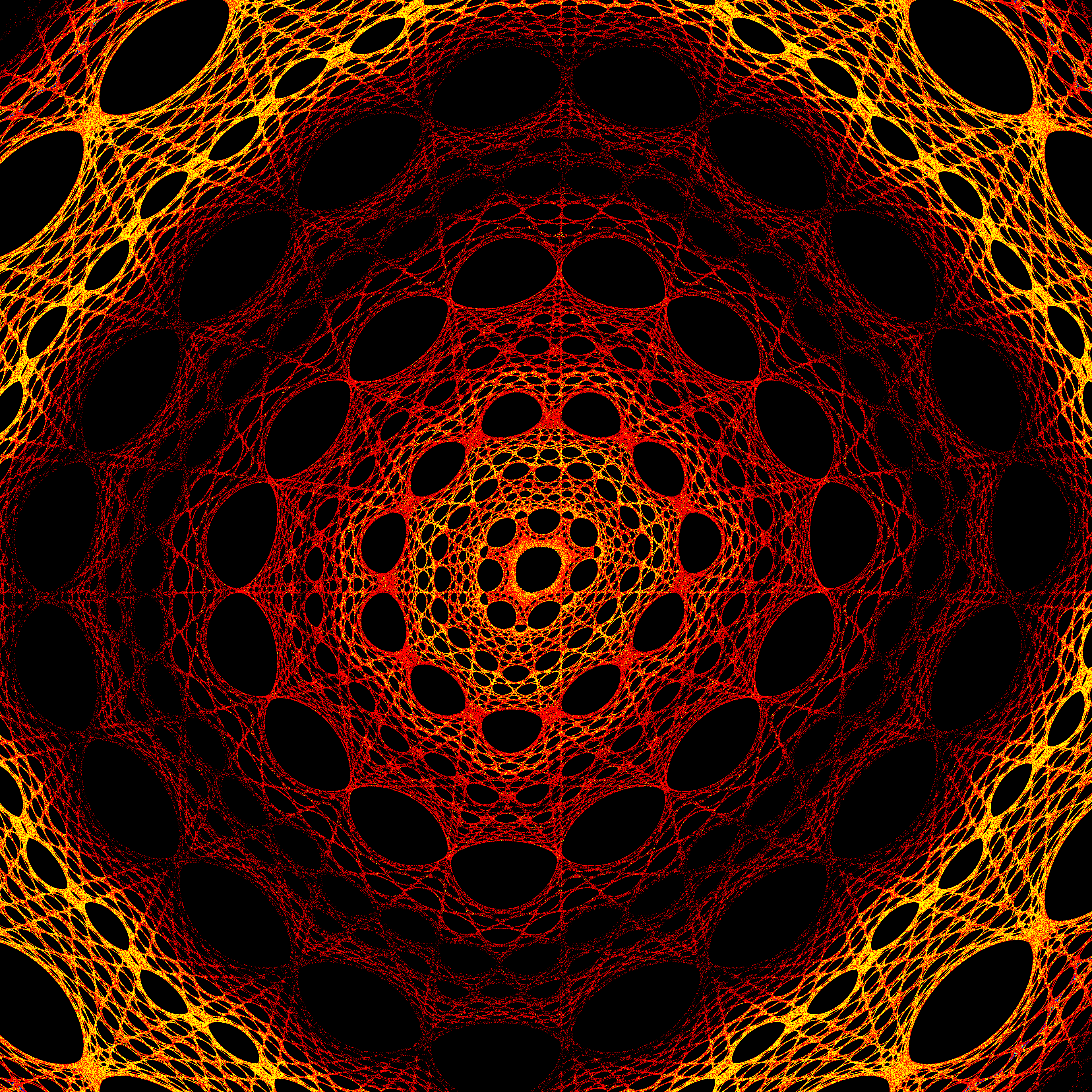
Table of Contents
1. Introduction
Barry Martin's "Hopalong" orbit fractals are a family of discrete-time dynamical systems:
- Classic Barry Martin fractal: \[ \begin{align*} x_{n+1} & = y_n - \mathrm{sgn}(x_n) \cdot \sqrt{\vert b x_n-c\vert} \\ y_{n+1} & = a-x_n \end{align*} \]
- Positive Barry Martin fractal: \[ \begin{align*} x_{n+1} & = y_n + \mathrm{sgn}(x_n) \cdot \sqrt{\vert b x_n-c\vert} \\ y_{n+1} & = a-x_n \end{align*} \]
- Additive Barry Martin fractal: \[ \begin{align*} x_{n+1} & = y_n + \sqrt{\vert b x_n-c\vert} \\ y_{n+1} & = a-x_n \end{align*} \]
- Sinusoidal Barry Martin fractal: \[ \begin{align*} x_{n+1} & = y_n + \sin{(b x_n-c)} \\ y_{n+1} & = a-x_n \end{align*} \]
All of these maps, and others, may be constructed from the following system as special cases: \[ \begin{align*} x_{n+1} & = y_n+d \cdot \mathrm{ssgn}(x_n) \cdot \left(f \cdot \sqrt{\vert b x_n-c\vert} + g \cdot \sin{(b x_n-c)} + h \cdot \vert b x_n-c\vert \right) \\ y_{n+1} & = a-x_n \end{align*} \] Where \[ \mathrm{ssgn}(v) = \cases{ s & $v\lt 0$ \cr 1 & $v\ge 0$ } \] \[ \mathrm{sgn}(v) = \cases{ -1 & $v\lt 0$ \cr +1 & $v\ge 0$ } \]
Note the simplified form of the \(\mathrm{sgn}(v)\) function used – the standard definition may be used for nearly identical results.
Some special cases:
- When \( d=-1, s=-1, f=1, g=0, h=0 \), the map becomes the "Classic Barry Martin fractal"
- When \( d=1, s=-1, f=1, g=0, h=0 \), the map becomes the "Positive Barry Martin fractal"
- When \( d=1, s=1, f=1, g=0, h=0 \), the map becomes the "Additive Barry Martin fractal"
- When \( d=1, s=1, f=0, g=1, h=0, c=0 \), the map becomes the "Sinusoidal Barry Martin fractal"
- When \( d=1, s=1, f=0, g=0, h=1, c=0 \), the map becomes the "The Gingerbread Man": \[ \begin{align*} x_{n+1} & = y_n + \sin{(b x_n)} \\ y_{n+1} & = a-x_n \end{align*} \]
- When \( d=1, s=1, f=0, g=0, h=1, c\ne0 \), the map becomes the "The Shifted Gingerbread Man": \[ \begin{align*} x_{n+1} & = y_n + \sin{(b x_n-c)} \\ y_{n+1} & = a-x_n \end{align*} \]
2. Algorithms
Just as with the Peter de Jong attractors we look at the probability density function, \(P(x,y)\), defined by the probability that some \((x_n, y_n)\) from the map will be in a neighborhood of \((x,y)\). While that sounds complicated, producing a visualization of this PDF is quite simple in practice – we simply visualize a histogram based on computed values of the map. The first step is to define a rectangular region of the plane over which we wish to visualize the PDF, and then define a set of discrete pixels over that region. Then we compute a few million, or billion, iterations of the map, and count the number of times we hit each pixel.
#include "ramCanvas.hpp"

std::vector<std::array<double, 14>> params {
  /*        a         b         c       d,      s,   f,   g,   h,     n,   k, x-min, x-max,  y-min, y-max */
  {  -2.00000, -0.33000,  0.01000,   -1.0,   -1.0, 1.0, 0.0, 0.0, 4.0e7, 1.0, -18.0,  17.0,  -18.0,  17.0}, //  0
  {   0.40000,  1.10000,  0.00000,   -1.0,   -1.0, 1.0, 0.0, 0.0, 2.5e7, 1.0,  -7.0,   7.0,   -7.0,   7.0}, //  1
  {  -3.14000,  0.20000,  0.30000,   -1.0,   -1.0, 1.0, 0.0, 0.0, 3.0e7, 1.0, -40.0,  40.0,  -40.0,  40.0}, //  2
  {  -3.14000,  0.19000,  0.32000,    1.0,   -1.0, 1.0, 0.0, 0.0, 1.0e7, 1.0, -38.0,  35.0,  -38.0,  35.0}, //  3
  {  -2.14000, -0.20000,  0.30000,    1.0,    1.0, 1.0, 0.0, 0.0, 3.0e7, 0.5,  -9.0,   7.0,   -9.0,   7.0}, //  4
  {   0.40000,  1.00000,  0.00000,   -1.0,   -1.0, 0.0, 1.0, 0.0, 2.0e6, 1.0, -70.0,  70.0,  -70.0,  70.0}, //  5
  {  -3.14000,  0.20000,  0.30000,   -1.0,   -1.0, 0.0, 1.0, 0.0, 6.0e7, 1.0, -45.0,  45.0,  -45.0,  45.0}, //  6
  {  -3.14000,  0.20000,  0.30000,    1.0,   -1.0, 0.0, 1.0, 0.0, 1.0e7, 1.0, -35.0,  35.0,  -35.0,  35.0}, //  7
  {  -2.00000, -0.33000,  0.01000,   -1.0,   -1.0, 1.0, 0.0, 1.0, 4.0e7, 1.0, -25.0,  25.0,  -25.0,  25.0}, //  8
  {  -3.14000,  0.20000,  0.30000,   -1.0,   -1.0, 1.0, 0.0, 1.0, 4.0e7, 1.0, -60.0,  60.0,  -60.0,  60.0}, //  9
  {  -3.14000,  0.20000,  0.30000,    1.0,   -1.0, 1.0, 0.0, 1.0, 6.0e7, 1.0, -90.0,  90.0,  -90.0,  90.0}, // 10
  {  -3.14000,  0.20000,  0.30000,   -1.0,   -1.0, 0.0, 0.0, 1.0, 2.0e7, 1.0, -17.0,  15.0,  -17.0,  15.0}, // 11
  {  -3.14000,  0.20000,  0.30000,    1.0,   -1.0, 0.0, 0.0, 1.0, 3.0e7, 1.0, -17.0,  14.0,  -17.0,  14.0}, // 12
  {  -3.14000,  0.20000,  0.30000,    1.0,   -1.0, 0.0, 0.0, 1.0, 1.0e7, 1.0, -17.0,  14.0,  -17.0,  14.0}, // 13
  {  -1.14000,  0.01000,  0.05000,    1.0,   -1.0, 0.0, 0.0, 1.0, 5.0e6, 1.0,  -3.5,   2.5,   -3.5,   2.5}, // 14
  {  -1.14000,  0.10000,  0.50000,    1.0,   -1.0, 0.0, 0.0, 1.0, 6.0e7, 1.0, -17.0,  14.0,  -17.0,  14.0}, // 15
};

int main(void) {
  std::chrono::time_point<std::chrono::system_clock> startTime = std::chrono::system_clock::now();
  const int BSIZ = 480*8;
  mjr::ramCanvas1c16b::colorType aColor;
  aColor.setChans(1);

  for(decltype(params.size()) j=0; j<params.size(); ++j) {
    mjr::ramCanvas1c16b theRamCanvas(BSIZ, BSIZ, params[j][10], params[j][11], params[j][12], params[j][13]);

    double a = params[j][0];
    double b = params[j][1];
    double c = params[j][2];
    double d = params[j][3];
    double s = params[j][4];
    double k = params[j][9];

    double f = params[j][5];
    double g = params[j][6];
    double h = params[j][7];

    /* Draw the Attractor on a 16-bit, greyscale canvas such that the level is the hit count for that pixel.
       Thus we are using an "image" as a way to store field data instead of color information. */
    double x        = 0.0;
    double y        = 0.0;
    uint64_t maxII  = 0;
    uint64_t inCnt  = 0;
    uint64_t maxItr = static_cast<uint64_t>(params[j][8]);
    uint64_t iPrt   = maxItr / 5;
    for(uint64_t i=1;i<maxItr;i++) {
      double xNew = y+d*(x<0.0?s:1.0)* (f*std::sqrt(std::abs(b*x-c)) + g*std::sin(b*x-c) + h*std::abs(b*x-c));
      double yNew = a-x;
      if ( !theRamCanvas.isCliped(x, y)) {
        inCnt++;
        theRamCanvas.drawPoint(x, y, theRamCanvas.getPxColor(x, y).tfrmAdd(aColor));
        if(theRamCanvas.getPxColor(x, y).getC0() > maxII) {
          maxII = theRamCanvas.getPxColor(x, y).getC0();
          if(maxII > 16384) { // 1/4 of max possible intensity
            std::cout << "ITER(" << j <<  "): " << i << " MAXS: " << maxII << " EXIT: Maximum image intensity reached" << std::endl;
            break;
          }
        }
      }
      if((i % iPrt) == 0)
        std::cout << "ITER(" << j <<  "): " << i << " MAXS: " << maxII << " INC: " << inCnt << std::endl;
      x=xNew;
      y=yNew;
    }
    std::cout << "ITER(" << j <<  "): " << "DONE" << " MAXS: " << maxII << " INC: " << inCnt << std::endl;

    // Log image transform
    theRamCanvas.applyHomoPixTfrm(&mjr::ramCanvas1c16b::colorType::tfrmLn1);
    maxII = static_cast<uint64_t>(std::log(static_cast<double>(maxII)));

    /* Create a new image based on csCCfractal0RYBCW -- this one is 24-bit RGB color. */
    mjr::ramCanvas3c8b anotherRamCanvas(BSIZ, BSIZ);
    typedef mjr::ramCanvas3c8b::colorType::csCCfractal0RYBCW cs_t;
    for(int yi=0;yi<theRamCanvas.getNumPixY();yi++)
      for(int xi=0;xi<theRamCanvas.getNumPixX();xi++)
        anotherRamCanvas.drawPoint(xi, yi, cs_t::c(k * theRamCanvas.getPxColor(xi, yi).getC0() / static_cast<mjr::ramCanvas3c8b::csFltType>(maxII)));

    anotherRamCanvas.writeTIFFfile("barrymartin_" + mjr::math::str::fmt_int(j, 2, '0') + ".tiff");
  }
  std::chrono::duration<double> runTime = std::chrono::system_clock::now() - startTime;
  std::cout << "Total Runtime " << runTime.count() << " sec" << std::endl;
  return 0;
}
Source Link: barrymartin.cpp
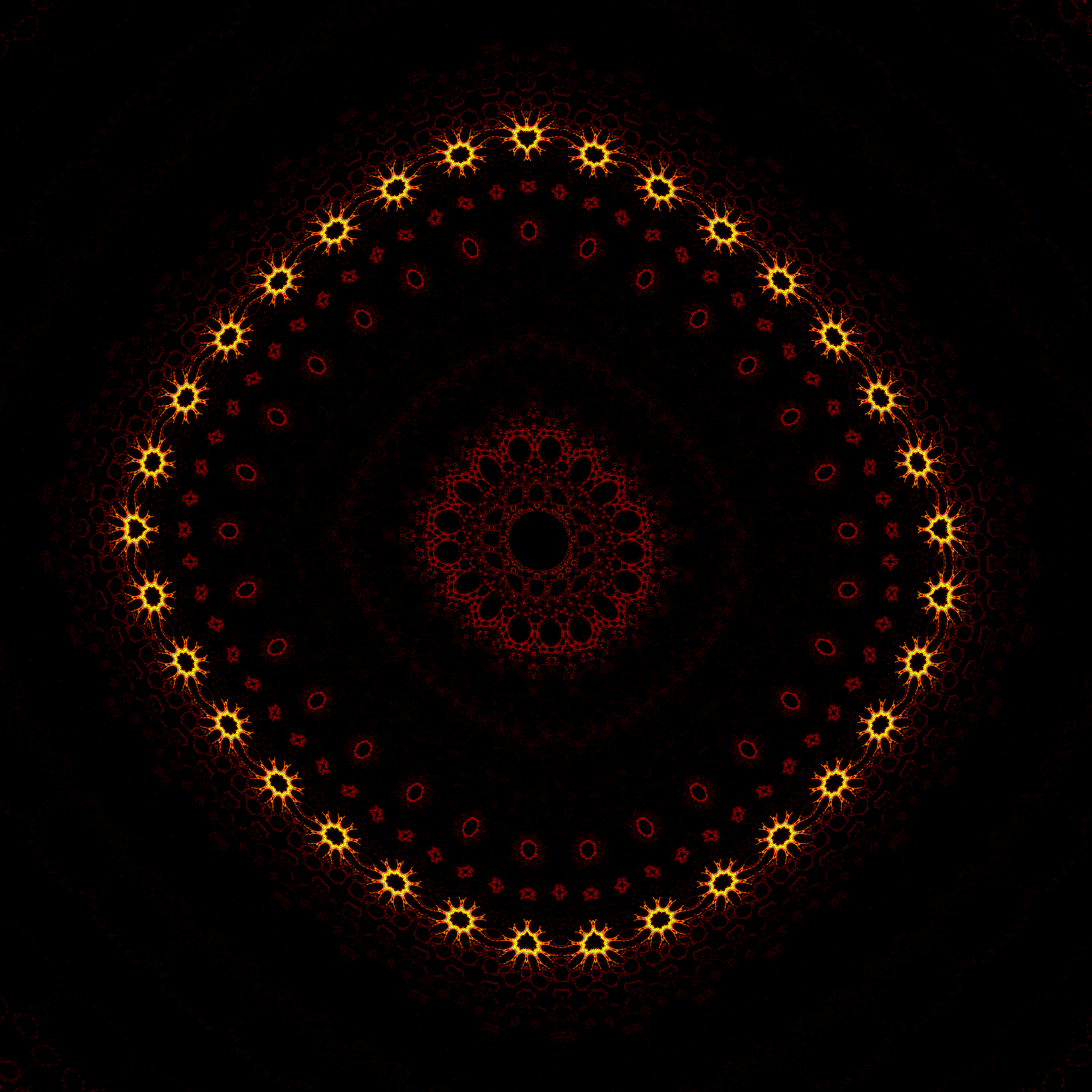
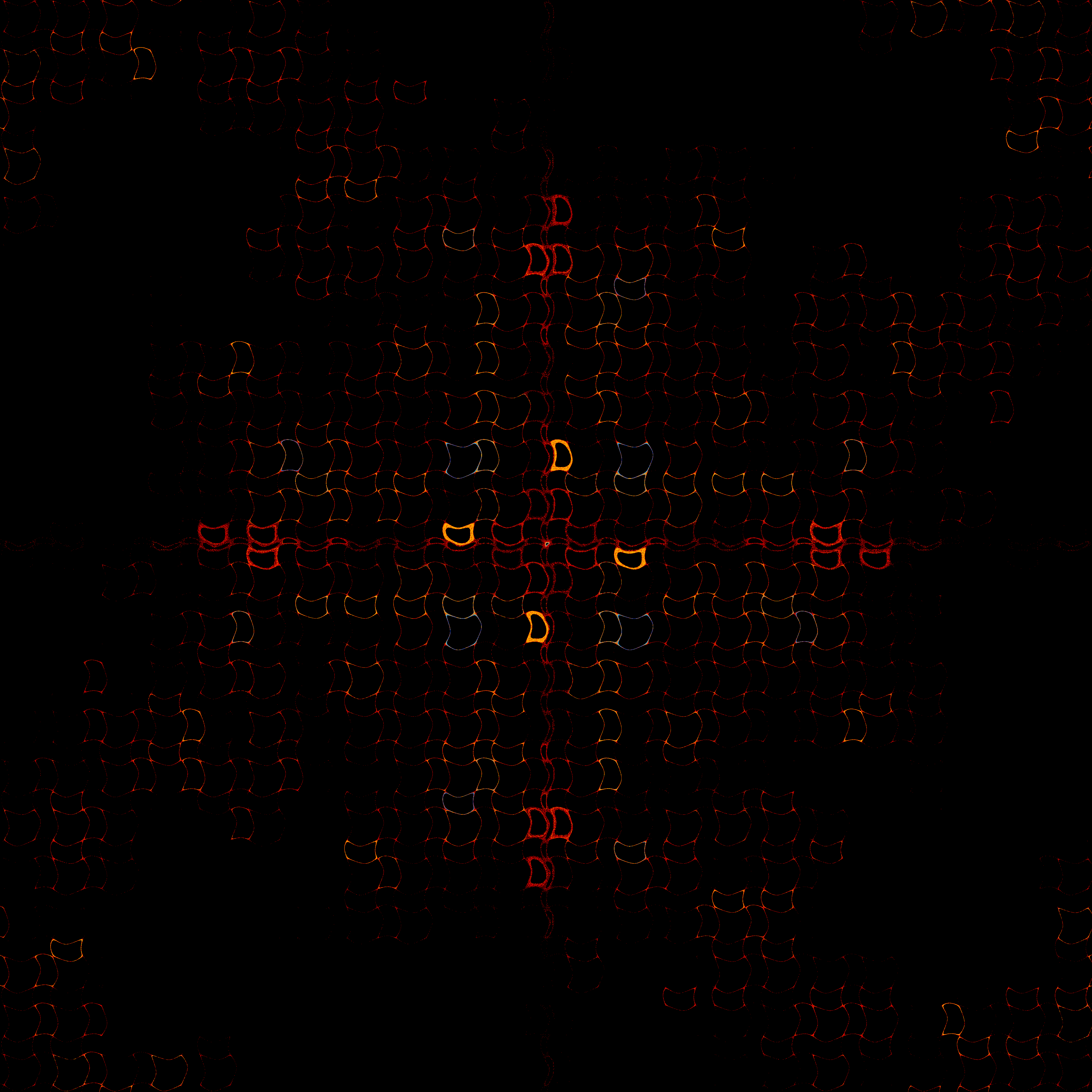
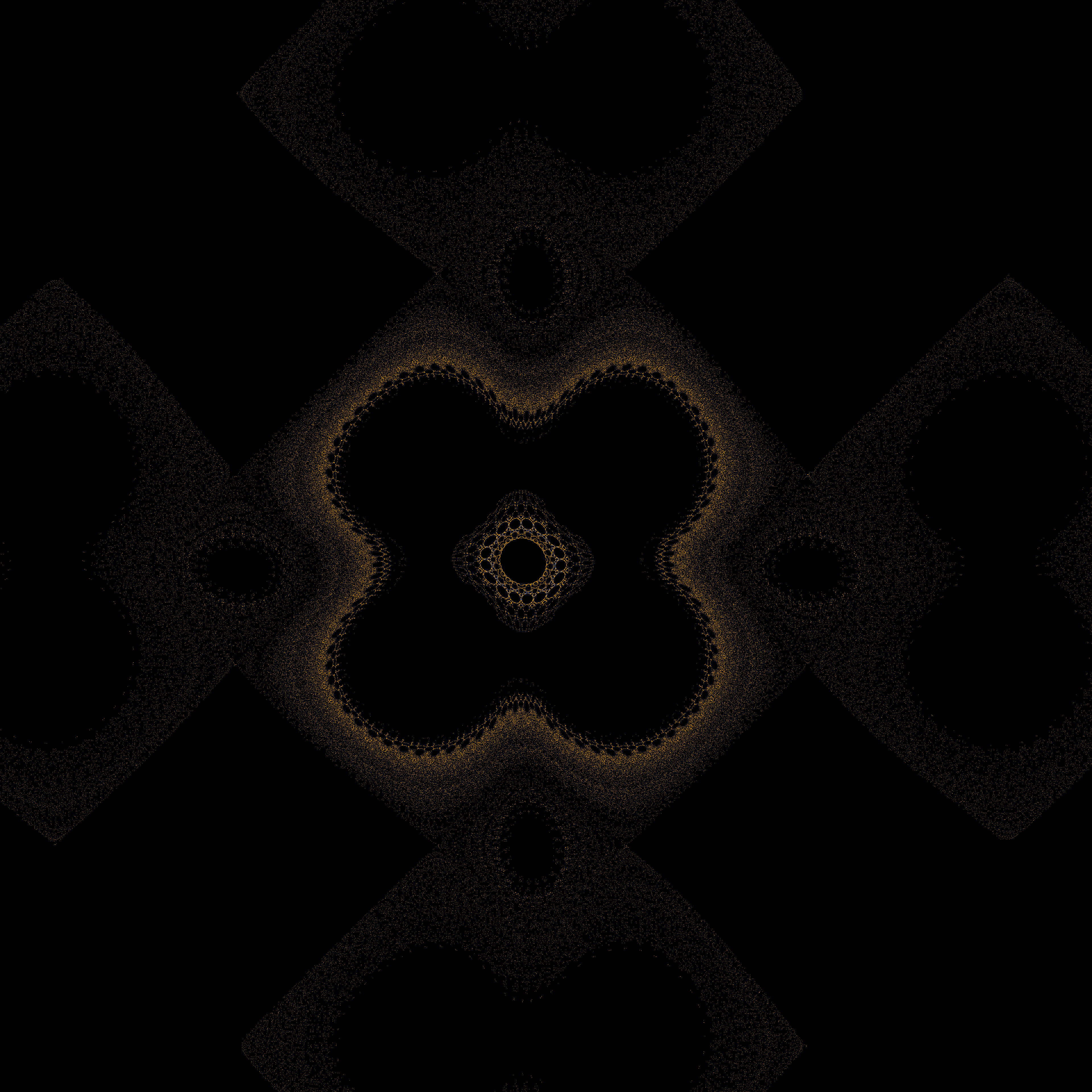
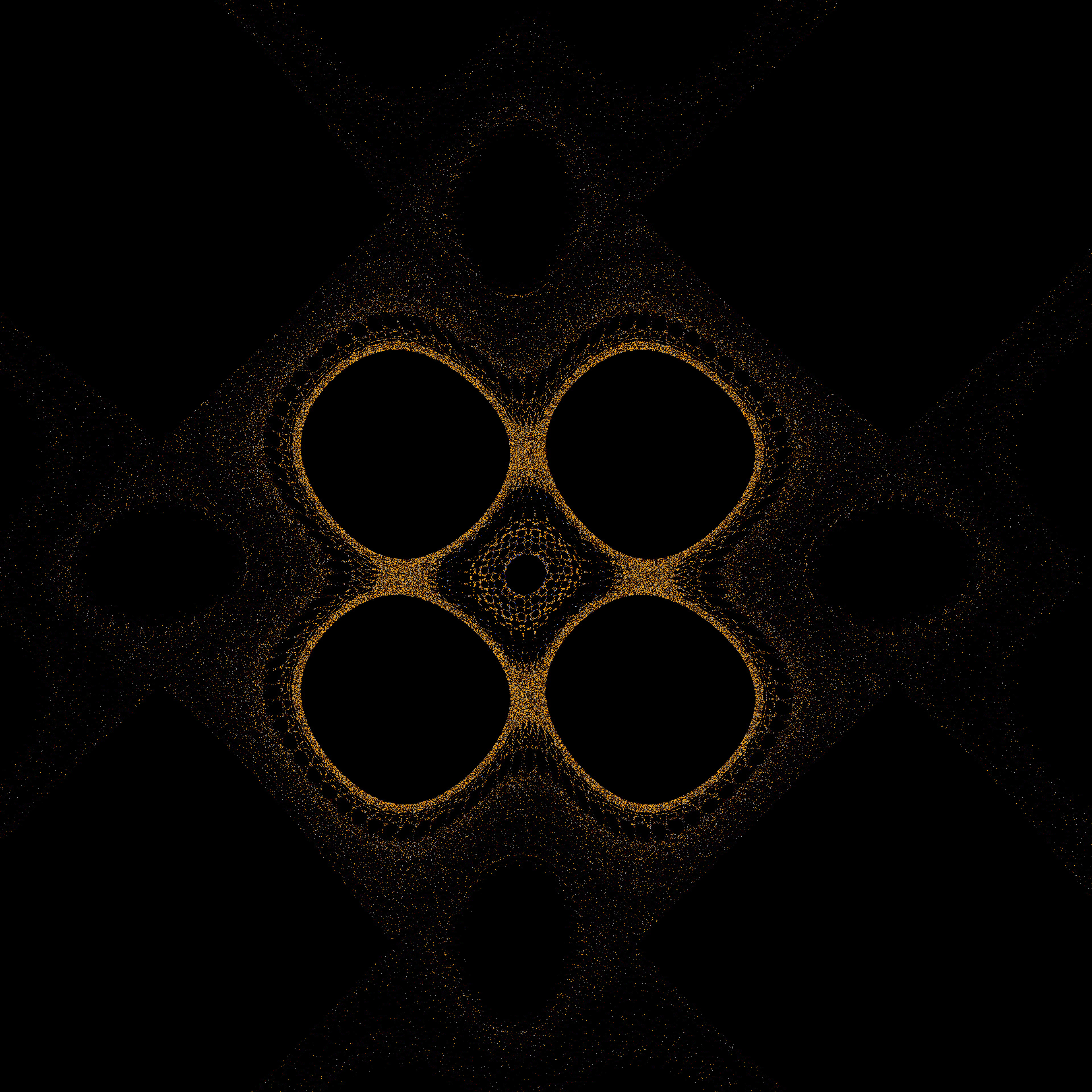
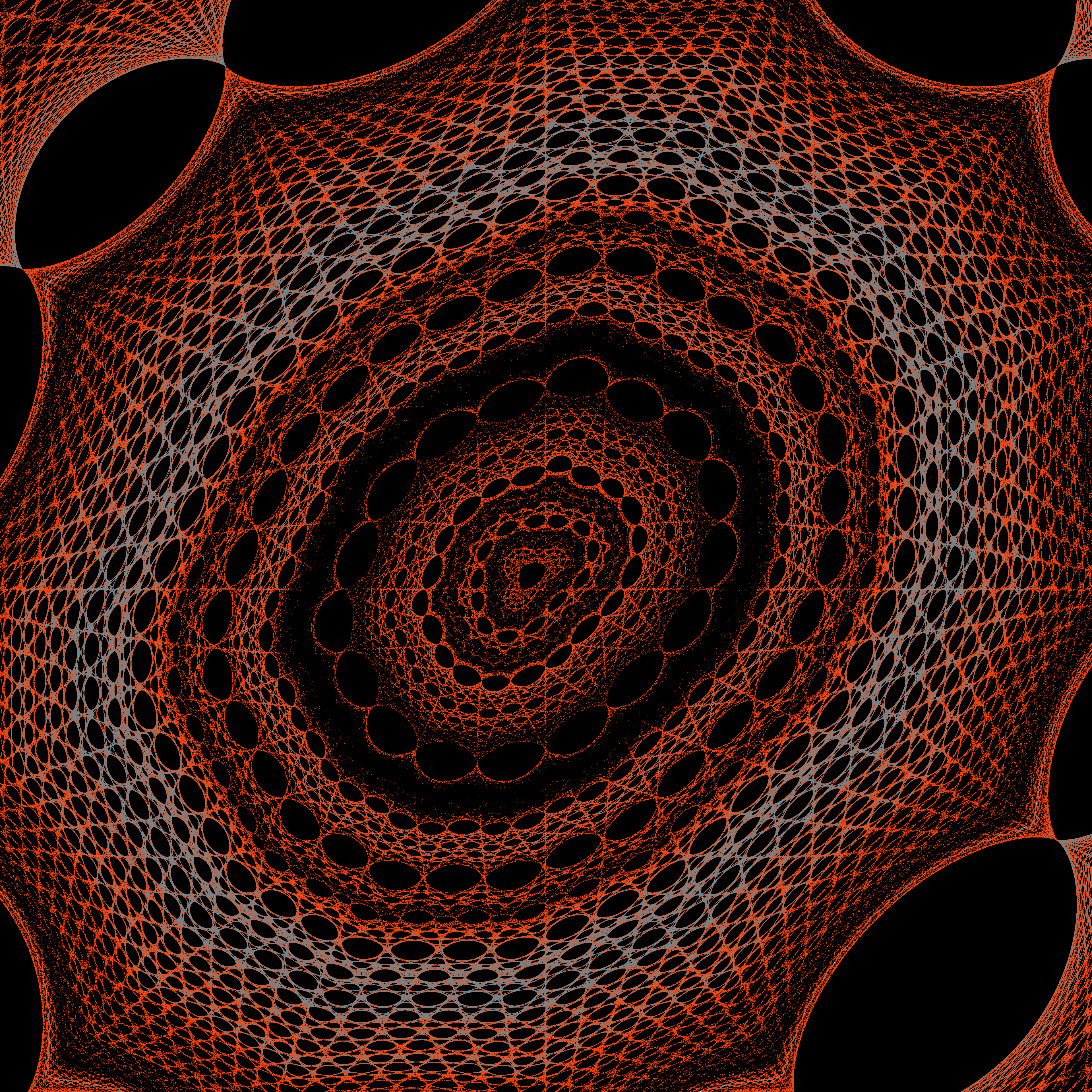
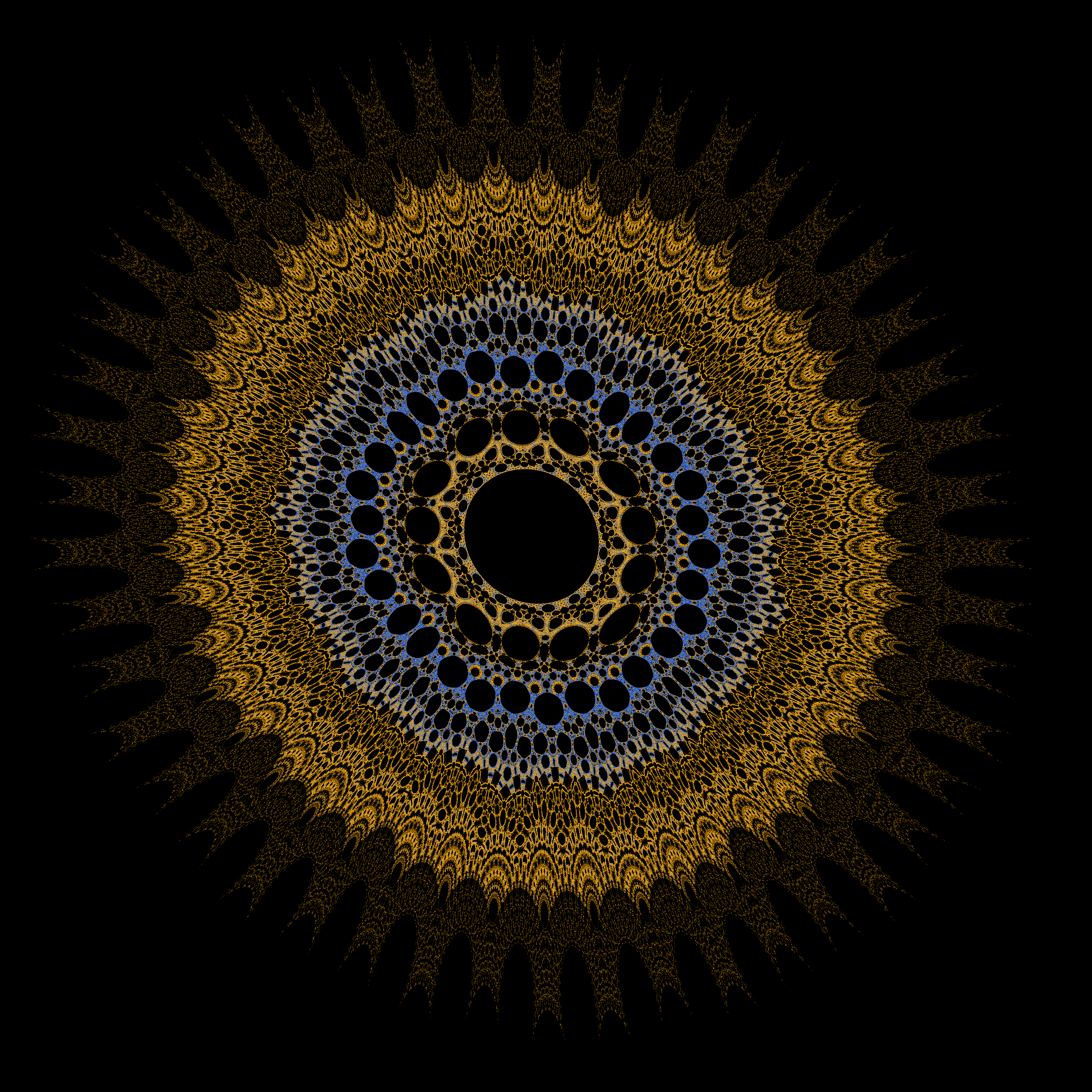
The above program will generate several images includeing the "Classic Barry Martin Atractor":
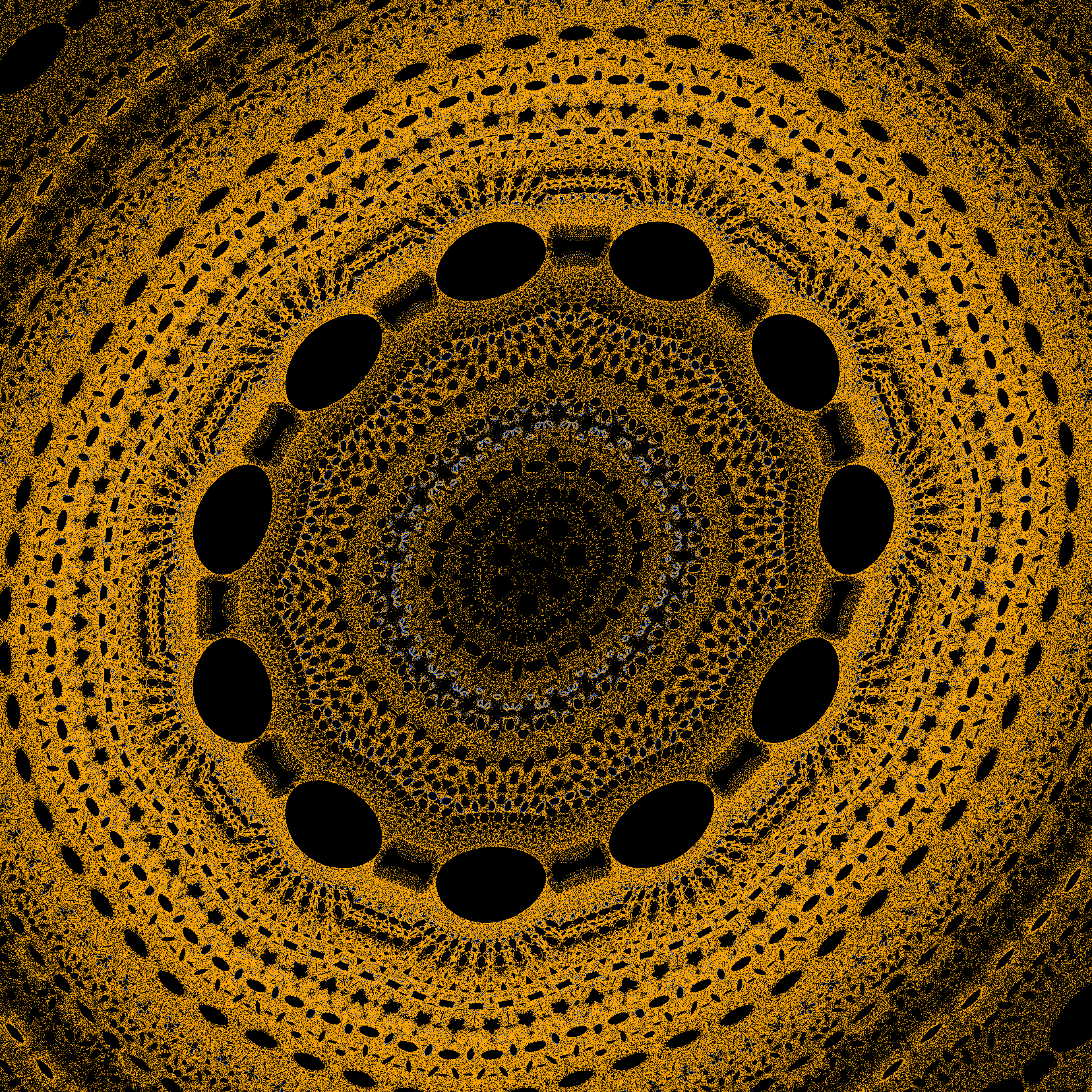
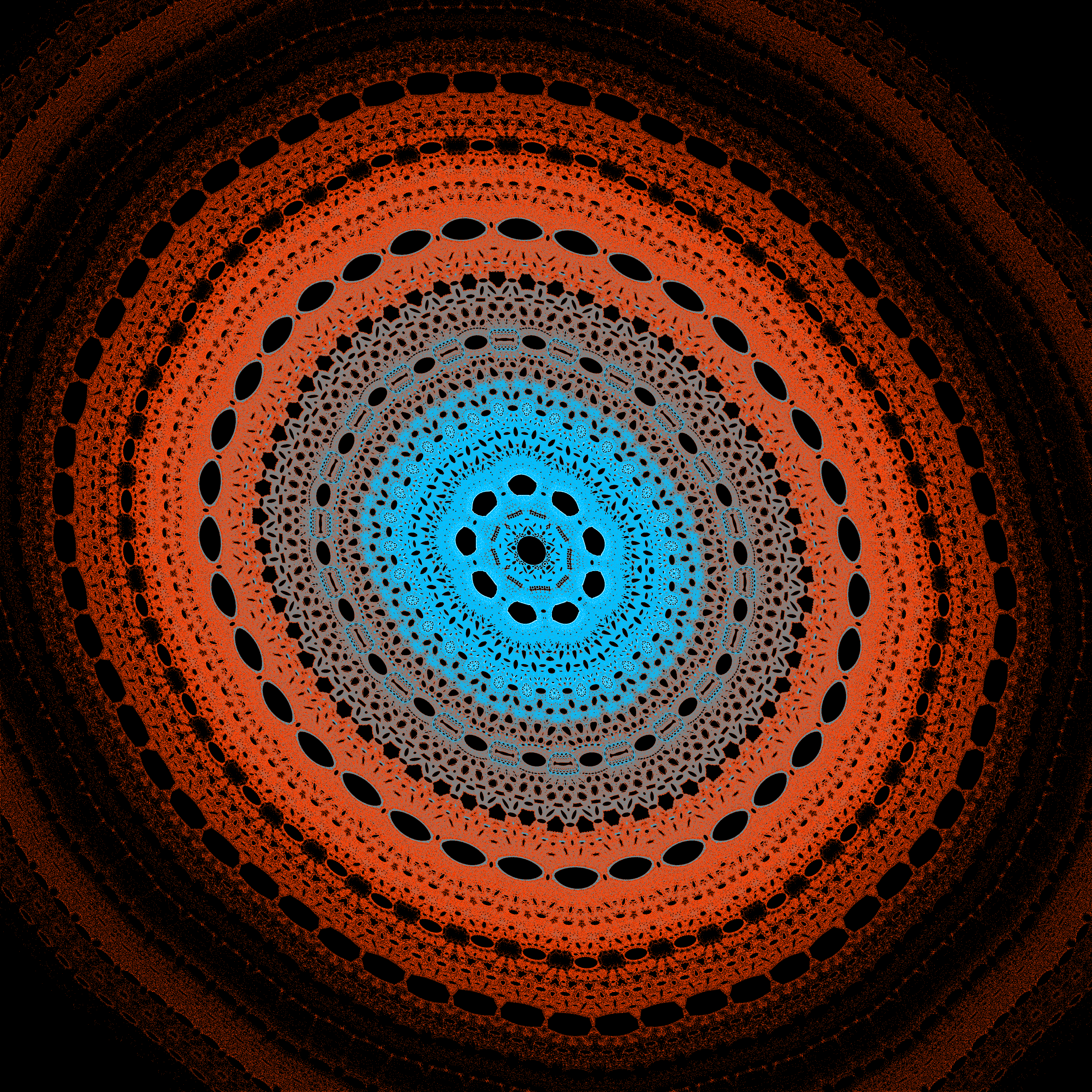
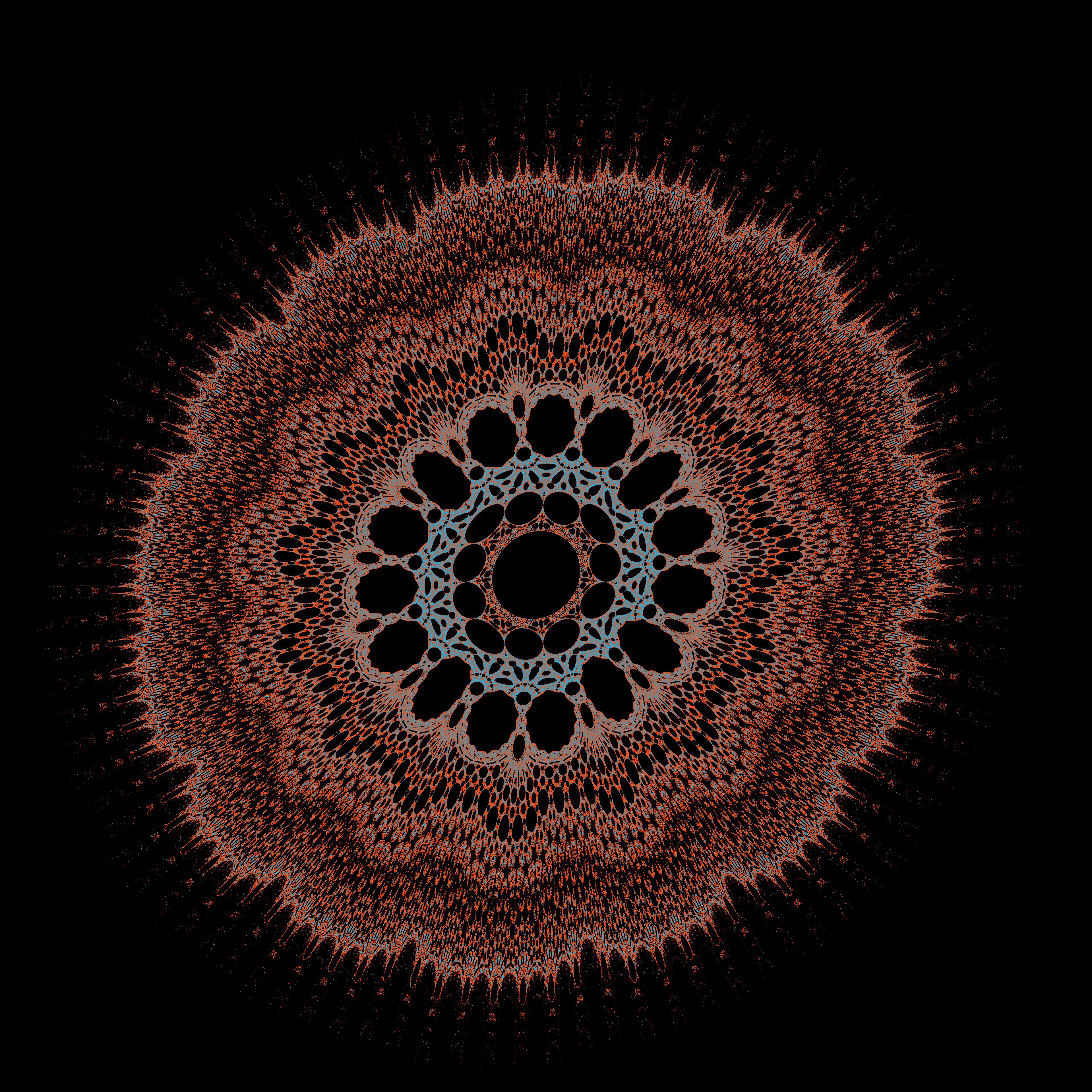
3. Gallery

4. References
- Martin, Barry. 1989. "Graphic Potential of Recursive Functions." In Computers in Art, Design and Animation, 109-29. Berlin, Heidelberg: Springer-Verlag.
- A. K. Dewdney. 1986. "Wallpaper for the Mind: Computer Images That Are Almost, but Not Quite, Repetitive." Scientific American, September, 12-23.
Check out the fractals section of my reading list.
All the code used to generate everything on this page may be found on github.